3. Power Analysis using DeclareDesign

There’s a lot that goes into research design, but here we focus on one thing that can be done well in R: power calculations. For this, I love DeclareDesign, a system to simulate Research Designs. Essentially, rather than plugging some parameters into a power calculator, you simulate your research and so investigate the statistical properties of your design. This is great, because it is often hard to include things like clustering and covariates in standard power calculators, and it forces you to be explicit about what you expect about your research.

This chapter will only scratch the surface of what you can do, so I really recommend further learning about DeclareDesign:

Read at least the slides before going forward!

This chapter covers power calculations in three designs: a simple comparison of means, a diff-in-diff design, and a matching design. To start of, we need example data. You can simulate this, but I prefer using existing data. Here we use Rhomis data.

Simple Power Calculation

The first design we consider is simply a comparison of means. We are interested in the effects of a project on the input of fertilizers.

Loading data

Here we take the Rhomis data, and add some variables. (For example, village codes: I create fake ones based on y-cooridnates.)

library(tidyverse)
library(DeclareDesign)
library(here)


n_clusters = 18

rhomis <-
  read_csv(here("data/RHoMIS_Indicators.csv")) %>% #names()
  filter(Country == "Burundi") %>% #count(Livestock_Orientation)

  # split the sample in villages, by lattitude
  filter(!is.na(GPS_LAT)) %>%
  arrange(GPS_LAT) %>%
  mutate(village = rep(1:n_clusters, each = nrow(.) / n_clusters , length.out =  nrow(.))) %>%
  # create some variables
  mutate(HFIAS_status = factor(HFIAS_status, levels = c("FoodSecure", "MildlyFI", "ModeratelyFI", "SeverelyFI")),
         food_secure = 1 * (as.numeric(HFIAS_status) <= 3),
         educated = 1*(Head_EducationLevel != "No_school"),
         female = 1* (HouseholdType == "woman_single")) %>%
  mutate(hh = row_number()) %>%
  select(!HFIAS_status) %>%

  # there are too many missings in my data; these seem reasonable to assume to be 0 when missing:
  mutate(across(c(LandOwned,NFertInput,educated),
         ~ if_else(is.na(.x),0,.x))) %>%
  select(village, hh, NFertInput, food_secure, educated, LivestockHoldings)

Declare Design

Now it’s time to start declaring our design. The first element of the design is the model, using declare_model() which essentially is my data. declare_model() follows the syntax of fabricate(): a package that is part of the DeclareDesign ecosystem that allows you to generate fake data. In this syntax, instead of using mutate() we can just supply new variables after a comma. In this case, I add potential outcomes, using potential_outcomes():

effect_size_simple <- 70

model_simple <- 
  declare_model(
    rhomis %>% select(village, NFertInput),
    potential_outcomes(Y ~ NFertInput + Z * effect_size_simple)
)

The potential outcomes are generated using potential_outcomes(). This will create two variables Y_Z_1 and Y_Z_0, which are the potential outcomes if having received treatment (Z == 1) or not. The difference between these is the effect size, which we assume to be 70 kg, we store this in a variable, so we can play with it later on. Note that I will generate Z in the next step.

Then it’s time to think about assignment. I do a clustered randomization, based on the villages:

assignment_simple <-
  declare_assignment(Z = cluster_ra(clusters = village, prob = 0.5))

Next, I declare my theoretical quantity of interest is the treatment effect in year 1. This is basically my research question.

inquiry_simple <-  
  declare_inquiry(ATE = mean(Y_Z_1 - Y_Z_0))

measurement_simple <- declare_measurement(
  Y = reveal_outcomes(Y ~ Z)
)

Since I won’t be able to observe Y_Z_1 for the control group, nor Y_Z_0 for the treatment group, I will need an estimation strategy. The below arguments will be put into lm_robust by default, and the term argument determines which coefficient is our estimate of interest:

estimator_simple <-
  declare_estimator(Y ~ Z,
                    clusters = village, 
                    inquiry = "ATE", 
                    term = "Z", 
                    label = "Simple")

Finally, I combine all these elements to declare my design. Note that it’s only here that R starts actually running the code to randomize things. The previous was just declaration!

design_simple <- model_simple + assignment_simple + inquiry_simple + measurement_simple + estimator_simple
summary(design_simple)

## 
## Research design declaration summary
## 
## Step 1 (model): declare_model(rhomis %>% select(village, NFertInput), potential_outcomes(Y ~ NFertInput + Z * effect_size_simple)) 
## 
## N = 290 
## 
## Added variable: village 
##  min median mean max   sd N_missing N_unique
##    1      9 9.44  18 5.23         0       18
## 
## Added variable: NFertInput 
##  min median  mean  max     sd N_missing N_unique
##    0     16 72.71 7500 465.79         0       44
## 
## Added variable: ID 
##  N_missing N_unique     class
##          0      290 character
## 
## Added variable: Y_Z_0 
##  min median  mean  max     sd N_missing N_unique
##    0     16 72.71 7500 465.79         0       44
## 
## Added variable: Y_Z_1 
##  min median   mean  max     sd N_missing N_unique
##   70     86 142.71 7570 465.79         0       44
## 
## Step 2 (assignment): declare_assignment(Z = cluster_ra(clusters = village, prob = 0.5)) 
## 
## Added variable: Z 
##     0    1
##   146  144
##  0.50 0.50
## 
## Step 3 (inquiry): declare_inquiry(ATE = mean(Y_Z_1 - Y_Z_0)) -------------------
## 
## A single draw of the inquiry:
##  inquiry estimand
##      ATE       70
## 
## Step 4 (measurement): declare_measurement(Y = reveal_outcomes(Y ~ Z)) ----------
## 
## Added variable: Y 
##  min median   mean  max     sd N_missing N_unique
##    0     70 107.46 7500 464.29         0       56
## 
## Step 5 (estimator): declare_estimator(Y ~ Z, clusters = village, inquiry = "ATE", term = "Z", label = "Simple") 
## 
## Formula: Y ~ Z 
## 
## A single draw of the estimator:
##  term estimator  estimate std.error  statistic   p.value  conf.low conf.high
##     Z    Simple -4.859351  58.40995 -0.0831939 0.9347302 -128.6916  118.9729
##        df outcome inquiry
##  15.98618       Y     ATE

Diagnosing Design and calculating power

If you want to browse a version of the data created by your design, use the draw_data() function. This is useful to examine the properties of the data.

draw_data(design_simple) %>%
  as_tibble()

## # A tibble: 290 × 7
##    village NFertInput ID    Y_Z_0 Y_Z_1     Z     Y
##      <int>      <dbl> <chr> <dbl> <dbl> <int> <dbl>
##  1       1          5 001       5    75     0     5
##  2       1         26 002      26    96     0    26
##  3       1         40 003      40   110     0    40
##  4       1          0 004       0    70     0     0
##  5       1         10 005      10    80     0    10
##  6       1         25 006      25    95     0    25
##  7       1         25 007      25    95     0    25
##  8       1         60 008      60   130     0    60
##  9       1          0 009       0    70     0     0
## 10       1          0 010       0    70     0     0
## # ℹ 280 more rows

Now to calculate our power. The diagnose_design() will run our model 500 times and our power is simply the fraction of times we find a statistically significant effect.

set.seed(1)
diagnose_design(design_simple)

## 
## Research design diagnosis based on 500 simulations. Diagnosis completed in 5 secs. Diagnosand estimates with bootstrapped standard errors in parentheses (100 replicates).
## 
##         Design Inquiry Estimator Outcome Term N Sims Mean Estimand
##  design_simple     ATE    Simple       Y    Z    500         70.00
##                                                             (0.00)
##  Mean Estimate   Bias SD Estimate   RMSE  Power Coverage
##          72.34   2.34       60.30  60.29   0.27     1.00
##         (2.84) (2.84)      (0.82) (0.80) (0.02)   (0.00)

Our power is 0.23, meaning we found a significant result in 23% of our model runs. That’s way lower than the traditional 80% threshold.

How large should our effect size be to reach a power of 0.8? We can use the redesign() function for this. Redesign allows you to vary certain parameters of your design, and run the design 500 times for each value of the parameter. You can change this number using the sims argument.

num_sims <- 500

set.seed(1)
diagnosis_simple <-
  design_simple %>%
  redesign(effect_size_simple = seq(100,300,50)) %>%
  diagnose_design(sims = num_sims) %>%
  tidy() %>%
  as_tibble()

Now, I want a nice plot. For this I filter the tibble I created, and pipe it into ggplot():

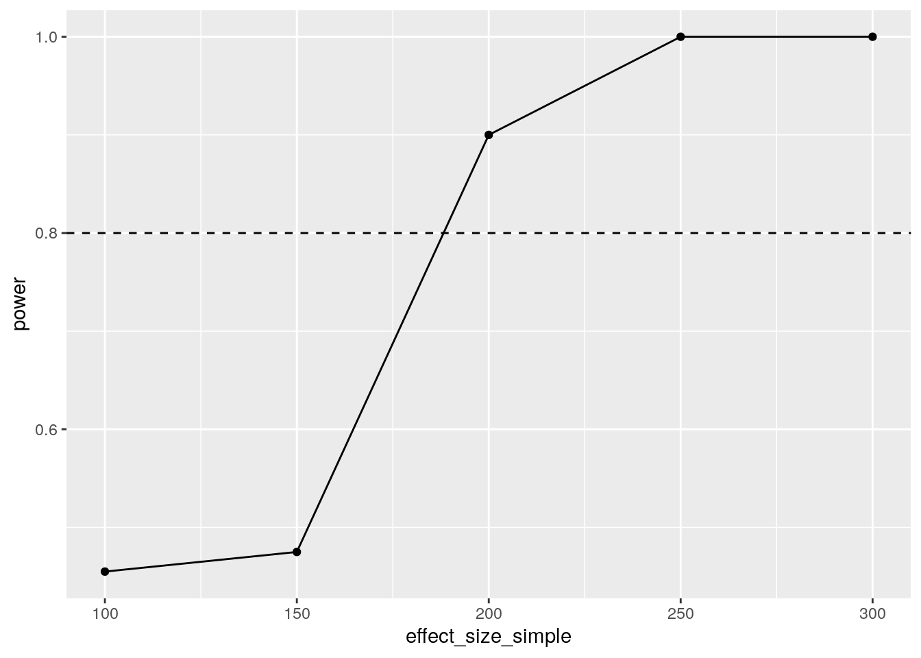
diagnosis_simple %>%
  filter(diagnosand == "power") %>%
  select(effect_size_simple,power = estimate) %>%
  ggplot(aes(x = effect_size_simple, y = power)) +
    geom_line() +
    geom_point() +
    geom_hline(yintercept=0.8,linetype=2)

We can reliably detect an effect size between 150 and 200 kgs of fertilizer. The mean fertilizer use is 70kg, so that seems unlikely to be realistic. Perhaps we can increase power using a diff-in-diff design?

Dif in diff

We have one round of data, so to analyze a diff in diff, we would have to simulate data. The key reason why a diff in diff design would matter, is because the outcomes are correlated between years, which should reduce standard errors and increase power.

So first order of business is to figure out how we can generate values for year 1 that are correlated to year 0, by a coefficient that we can vary so we can investigate the properties of our design.

Here’s what I’ve got (so far), a function that takes a vector, converts it to normal space, generates something correlated and maps it back:

correlate_var <- function(x, rho) {

  n <- length(x)

  # convert X to normal scores
  u  <- rank(x) / (n + 1)     # empirical CDF
  z1 <- qnorm(u)              # normal scores

  # generate correlated normal
  z2 <- rho * z1 + sqrt(1 - rho^2) * rnorm(n)

  # transform back
  u2 <- pnorm(z2)

  # map onto original distribution
  x_sorted <- sort(x)
  y <- quantile(x_sorted, probs = u2, type = 8)
  y
}

I update my design accordingly, by generating the second year. For that, I prefer to use dplyr, but it should be possible with fabricate() as well. I first rename all our time-variant varaible to have _0 at the end, create a correlated varaible with _1 at the end, and then pivot_longer.

effect_size_dd <- 70
sd_dd <- 100
rho_dd <- 0.7
model_dd <- declare_model(

  rhomis %>%
    select(village, NFertInput) %>%
    # add one more year
    rename_with(~ paste0(., "_0"), -village) %>%
    mutate(
      NFertInput_1 = correlate_var(NFertInput_0, rho_dd)
    ) %>%
    pivot_longer(
      ends_with(c("_0","_1")), 
      names_to = c(".value", "t"),
      names_pattern = "(.*)_([0-9]+)$",
      values_drop_na = TRUE,
      names_transform = list(t = as.integer)
    ),
    potential_outcomes(Y ~ NFertInput + Z * effect_size_dd)


)

I modify the inquiry and assignment to only take into account t == 1

inquiry_dd <-  
  declare_inquiry(ATE = mean(Y_Z_1 - Y_Z_0), subset = (t == 1)) 

assignment_dd <-
  declare_assignment(treatment_group = cluster_ra(clusters = village, prob = 0.5),
                     Z = t * treatment_group)

Measurement is unchanged:

measurement_dd <- declare_measurement(
  Y = reveal_outcomes(Y~Z)

)

Then I use feols() from the fixest package to estimate a Two-way fixed effects (2FE) model. This can be easily extended to more complex designs (but beware!).

library(fixest)
library(broom)
 
estimator_dd <-
  declare_estimator(Y ~ Z | treatment_group + t,
                    cluster = "village",
                    .method = feols, 
                    term = "Z", 
                    inquiry = "ATE", 
                    label = "2FE")

The complete design is then:

design_dd <- model_dd + assignment_dd + inquiry_dd + measurement_dd + estimator_dd

Let’s have a look at our power now! Of course, in a DiD setting, power depends not only on the effect size, but also on how well the years correlate. I therefore also vary the rho_dd variable, which controls the correlation between fertilizer input in years 0 and 1:

set.seed(1)
diagnosis_dd <-
  design_dd %>%
  redesign(
    effect_size_dd = c(100, 150, 200),
    rho_dd = c(0.3,0.6, 0.9)
  ) %>%
  diagnose_design(sims = num_sims) %>%
  tidy() %>%
  as_tibble()

Putting it in a plot again:

diagnosis_dd %>%
  filter(diagnosand == "power") %>%
  rename(power = estimate) %>%
  mutate(rho_dd = factor(rho_dd)) %>%
  ggplot(aes(x = effect_size_dd, y = power, color = rho_dd, shape = rho_dd)) +
    geom_line() +
    geom_point() +
    geom_hline(yintercept=0.8, linetype=2)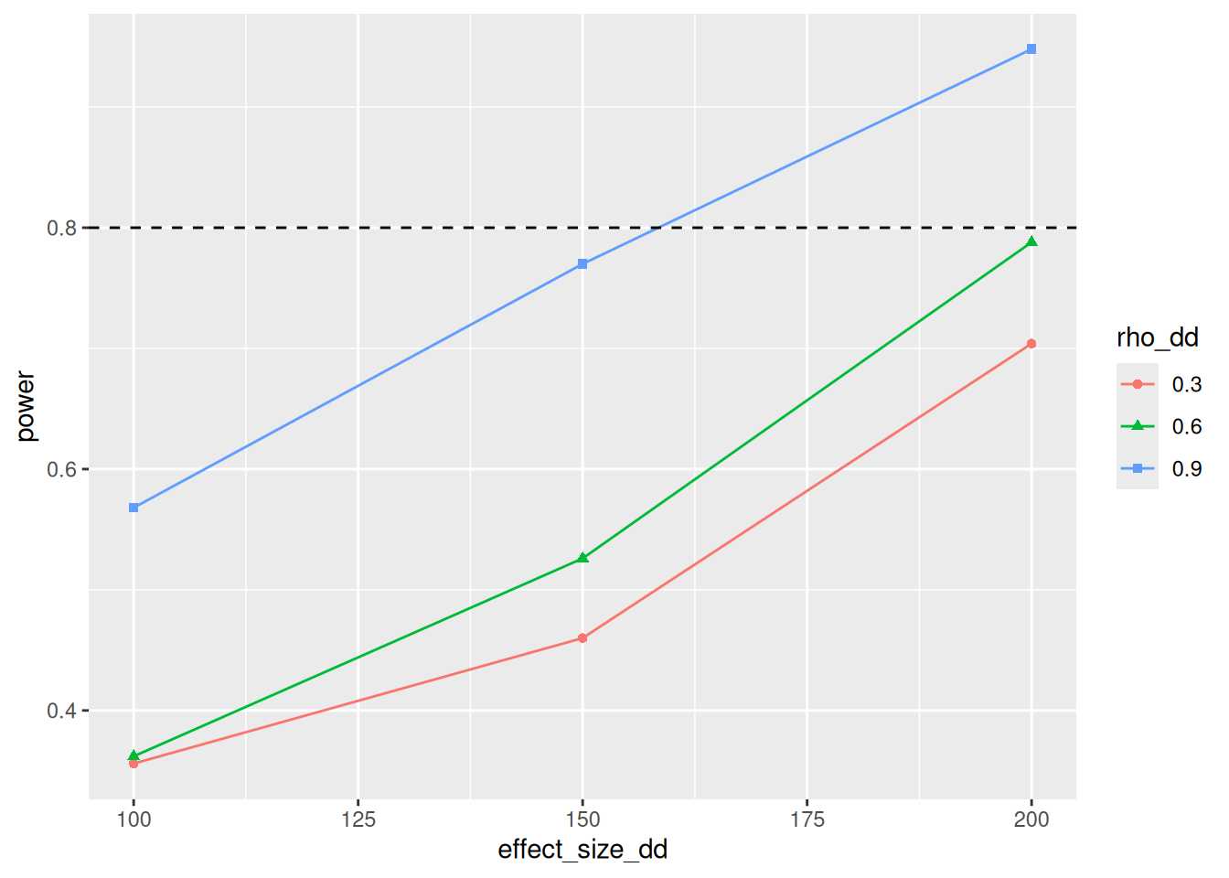

So at high levels of Rho, our power is slightly higher than when using the simple model. The lower rho is, the less added value the diff-in-diff model has. But honestly, I am suprised with how small the differences are.

Matching

Finally, let’s imagine a scenario where treatment isn’t random, but correlated to outcomes, so we would need matching.

Let’s also look at food_secure, since it’s binary, and thus adds a twist here and there.

Also, I will use the resample_data() function to pretend that we can visit more households than are in my original data set.

Declare Design

The first novel thing is the binary outcome. We want an easy to interpret effect size: a percentage point increase in food secure households. This is a bit trickey: before we just added the effect size to everyone. But for binary variables, we only change a 0 to a 1 for a certain share of the population. Let’s just define that first. The function below flips a certain number of 0s to 1, so that we have a nice effect size:

flip_zeroes <- function(x, Z, effect) {

    # how many 1s do we currently have?
    n_current_ones <- sum(x[Z == 1])

    # how many 1s should we have?
    p_current <- mean(x[Z == 1])
    p_target  <- p_current + effect
    n_target_ones  <- round(p_target * sum(Z == 1))
  
    # figure out which zeros to flip
    n_to_flip <- n_target_ones - n_current_ones
    
    # If nothing to flip, return x
    if (n_to_flip <= 0) return(x)
    
    zeros_index <- which(x[Z==1] == 0)
    
    # Can't flip more zeros than exist
    n_to_flip <- min(n_to_flip, length(zeros_index))
    if (n_to_flip == 0) return(x)
    
    flip_index <- sample(zeros_index, n_to_flip)

    # do it, and return the new x
    x[Z==1][flip_index] <- 1
    x
  }

Our model then becomes:

model_matching <- 
  declare_model(
    rhomis
  )

Then we do the assignment. This now consists of two steps:

Communities are assigned randomly, using cluster_ra()
Households are assigned in a way that is correlated with education and livestock holdings, (and also food_secure) using correlate().

rho <- 0.5

assignment_matching <- declare_assignment(
  hh_treat = correlate(
    given = educated * LivestockHoldings^2,
    rho = rho,
    draw_binomial,
    prob = 0.3
  ), 
  vill_treat = cluster_ra(clusters = village, prob = 0.5), 
  Z = hh_treat * vill_treat
)

Then we take an extra step: re-sampling.

Some notes:

We use resample_data() to sample more households than are in our original data set. The resulting data set will thus follow the same distribution as our original data, but with more observations.
In treatment communities, we only sample from treated households. In control communities, we don’t know who would have been treated, so we sample randomly.
We sample a certain number of households per community, which is a parameter we can vary in our diagnosis. The number differs between treatment and control communities, to allow oversampling the control observation to compensate for matching losses. To do this, we run the resample_data() function separately for treatment and control communities, using a combination of nest and map2 functions (see here).

communities_per_arm <- 10
respondents_treat <- 10
respondents_control <- 15

resample_hhs  <- function(df, communities_per_arm, respondents_treat, respondents_control){
  df %>% 
    filter(vill_treat == 0 | Z == 1) %>% 
    mutate(respondents = if_else(Z == 1, respondents_treat, respondents_control)) %>%
    nest(.by = c(Z, respondents)) %>%
    mutate(
      data = map2(
        data, 
        respondents, 
        ~resample_data(
          .x, 
          N = c(communities_per_arm,.y), 
          ID_labels = c("village", "hh"),
          unique_labels = TRUE
        )
      )
    ) %>% 
  unnest(data) 
}

resampling_matching <- declare_step(
  handler = resample_hhs,
  communities_per_arm = communities_per_arm,
  respondents_treat = respondents_treat,
  respondents_control = respondents_control
)

Measurement and inquiry are slightly different. I defined my treatment effects as a percentage point increase in food secure households. So if the percentage of food insecure households is very large relative to the effect size, the chance an individual household become food insecure is low. This messes with potential outcomes, as the effect on each individal depends on the means in the treatment group, and thus on the randomization. I therefore skip the potential outcomes, and just define my estimand as the effect size.

effect_size_matching <- 0.1

measurement_matching <-
 declare_measurement(
  Y = flip_zeroes(food_secure, Z, effect_size_matching)
)

inquiry_matching <- declare_inquiry(ATE = effect_size_matching)

Now for the estimators, let’s start with a simple one, with no matching:

estimator_matching_no_matching <- 
  declare_estimator(Y ~ Z, 
                    inquiry = "ATE", 
                    term = "Z", 
                    label = "Not matched",
                    cluster= village_unique)

Finally, I need to somehow put my matching model in DeclareDesign. Fortunately, you can put any the output of any function into the declare_estimator() function using the handler argument. It does need to accept a data argument, and output a tidy() dataframe.

My function custom_match() accepts a data frame, uses MatchIt to create a matched data set, I define a function that does that, and some labelling:

# the select function would conflict with dplyr
# this syntax requires R 4.0 or higher

library(MatchIt, exclude("select"))


custom_match <- function(data,
                         equation,
                         outcome = "Y", 
                         term = "Z", 
                         method = "nearest"){

  # the command filter(term == term) wouldn't do anything, so this is a workaround
  term_value <- term

  # run the matching model
  matchit_model <- matchit(equation,
                          data = data,
                         method = method)
  matched_df <- match.data(matchit_model)

  # run a regression, weighted by the propensity score
  lm_robust(Y ~ Z, data = matched_df, weights = weights, clusters = village_unique) %>%
    tidy() %>%
    mutate(outcome = outcome) %>%
    filter(term == term_value)
}

Then I add two estimator: one that uses PSM (‘nearest’) and one that uses CEM (‘cem’), so that we can compare these two matching methods in our diagnosis.

estimator_matching_psm <- declare_estimator(
  Z ~ educated + LivestockHoldings,
  handler = label_estimator(custom_match),
  inquiry = "ATE",  # Tie the estimator to the declared inquiry
  label = "Matched PSM",
  term = "Z",
)

estimator_matching_cem <- declare_estimator(
  Z ~ educated + LivestockHoldings,
  handler = label_estimator(custom_match),
  inquiry = "ATE",  # Tie the estimator to the declared inquiry
  label = "Matched CEM",
  term = "Z",
  method = "cem"
)

And let’s combine it into one design!

design_matching  <-
  model_matching +  assignment_matching +  resampling_matching + measurement_matching + 
  inquiry_matching + 
  estimator_matching_no_matching + estimator_matching_psm + estimator_matching_cem

Note that to explore this design and fine tune matching procedures, it may be useful to run draw_data() a few times.

Bias

First, let’s examine bias, given selection effects. The strength of the selection effect is given by rho, so I use redesign() to vary it:

set.seed(1)
diagnosis_matching_bias <-
  design_matching %>%
  redesign(rho = seq(from = 0, to = 0.75, by = 0.25))  %>%
  diagnose_design(sims = num_sims) %>%
  tidy() %>%
  as_tibble()

And I put the result in a plot:

diagnosis_matching_bias %>%
  filter(diagnosand == "bias") %>%
  select(rho, bias = estimate, estimator) %>%
  ggplot(aes(x = rho, y = bias, 
             shape = estimator, color=estimator)) +
    geom_line() +
    geom_point()

It’s clear that while PSM reduced bias, but CEM performed much better.

Power

Then, let’s examine power. I drop the no matching a psm, to save some simulation time.

design_cem  <-
  model_matching +  assignment_matching +  resampling_matching + measurement_matching + 
  inquiry_matching + 
  estimator_matching_cem


set.seed(1)
diagnosis_matched_power <-
  design_cem %>%
  redesign(
    communities_per_arm = c(5,30,50),
    effect_size_matching = c(0.01,0.2, 0.3)
  ) %>%
  diagnose_design(sims = num_sims) %>%
  tidy() %>%
  as_tibble()

So at 30 communities per arm, our design can pick up an effect of 0.3, but to pick up an effect of 0.2 we should ideally increase our sample.

diagnosis_matched_power %>% 
  filter(diagnosand == "power") %>%
  mutate(effect_size_matching = factor(effect_size_matching)) %>%
  select(communities_per_arm, power = estimate, estimator, effect_size_matching) %>%
  ggplot(aes(x = communities_per_arm, y = power, 
             shape = effect_size_matching, color=effect_size_matching)) +
    geom_line() +
    geom_point() +
    geom_hline(yintercept=0.8,linetype=2)